ECE 4160 Fast Robots
Raphael Fortuna
Lab reports made by Raphael Fortuna @ rafCodes Hosted on GitHub Pages — Theme by mattgraham
Home
Lab 7: Kalman Filter
Summary
In this lab, I made a Kalman Filter in Python and extrapolated ToF values. I first estimated the drag and momentum of the car to initialize the A and B matrix for the Kalman Filter. Then I found the process noise and sensor noise covariance matrixes. I then implemented and tested the Kalman filter in Python code to check my parameters and extrapolated ToF values as well to speed up estimated ToF sampling on my car.
Estimate Drag and Momentum Task
I first used a step response to create the ToF and PWM graphs needed to get the drag and momentum values for the Kalman Filter. I drove my car towards a wall and logged the motor PWM values and ToF sensor output. I set the PWM value for the step response to 85 as this was my maximum value for the PID in lab 6.
Here is my graph for calculating the rise time and steady state with ToF, PWM, and speed with the x axis in seconds. The second graph is annotated with the 90% rise time and steady state speed:
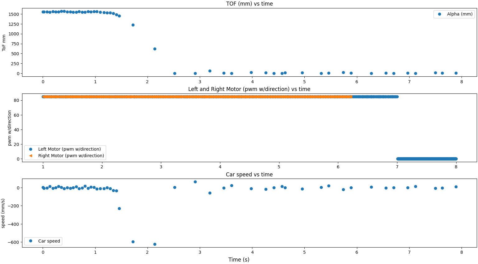
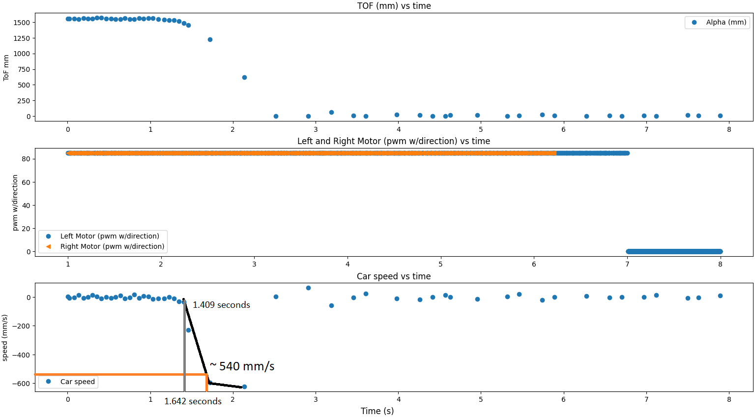
From this, I got that my steady state speed was ~600 mm/s. The 90% rise time was 0.2329 seconds.
Initialize KF Task
I first computed my A and B matrices and discretized them using the code below. My sampling time was 85 samples over 8 seconds for 0.094 seconds per sample.
Here is the initialization for the Kalman Filter class as well.
I used the C matrix provided in lecture and in the lab handout as seen below:
My discretized A, discretized B, and C matrices were:
- A: [[1.,0.094], [0., 0.07066123]]
- B: [[0.], [557.60325996]]
- C: [[-1., 0.]]
Next, I specified my process noise and sensor noise covariance matrices and calculated them using the code below. I used ballpark values for the variances as suggested, with each Kalman Filter output graph below having different variances.
I then initialized my state vector as seen below and started the loop for the Kalman filter.
When calculating the loop, I used the code provided in lecture, on the lab document, and the explanations provided on Anaya’s website found here. I made sure to normalize the input to 1 by dividing the PWM values by the maximum PWM value of 85.
I then ran the Kalman filter on PID data from lab 6 and plotted the results.
This ToF data from this data has some noise so it will be interesting to see how the variances modify the Kalman Filter's behavior with this outlier.
My first Kalman Filter output graph with the following variances:
- Process noise variance for distance: 10
- Process noise variance for speed: 10
- Sensor noise variance: 20
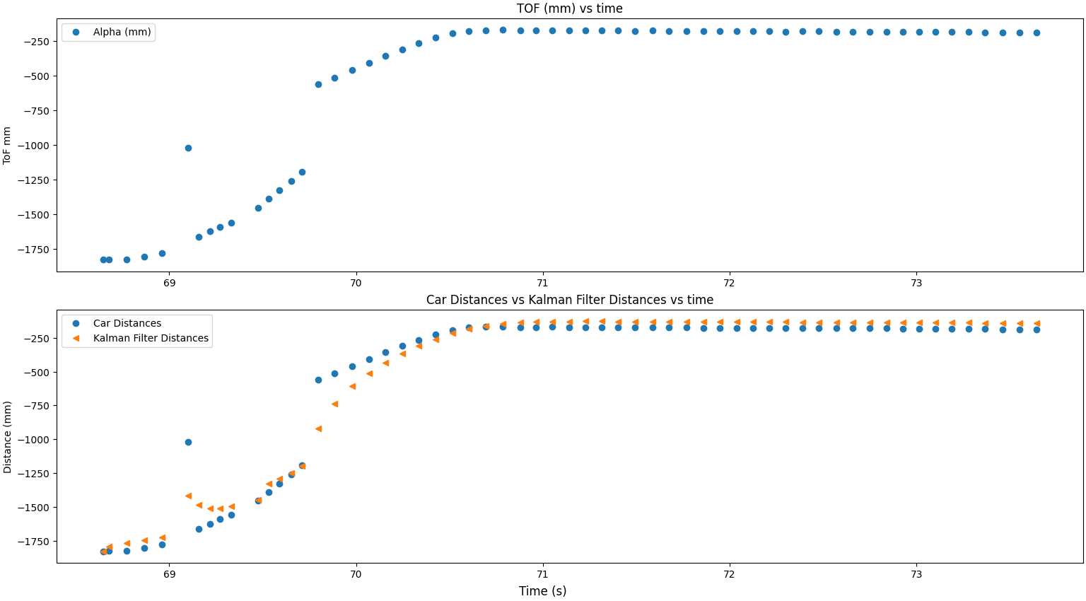
With these values, the sensor is trusted a little less, but the Kalman Filter still follows the noise in the ToF data.
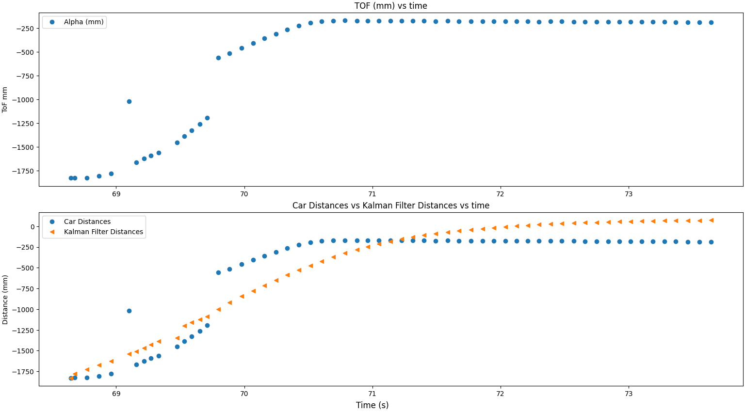
My second Kalman Filter output graph with the following variances:
- Process noise for distance: 10
- Process noise for speed: 10
- Sensor noise for the: 100
With these values, the sensor is trusted a lot less, and the Kalman Filter disregards the noise and smooths the ToF measurments.
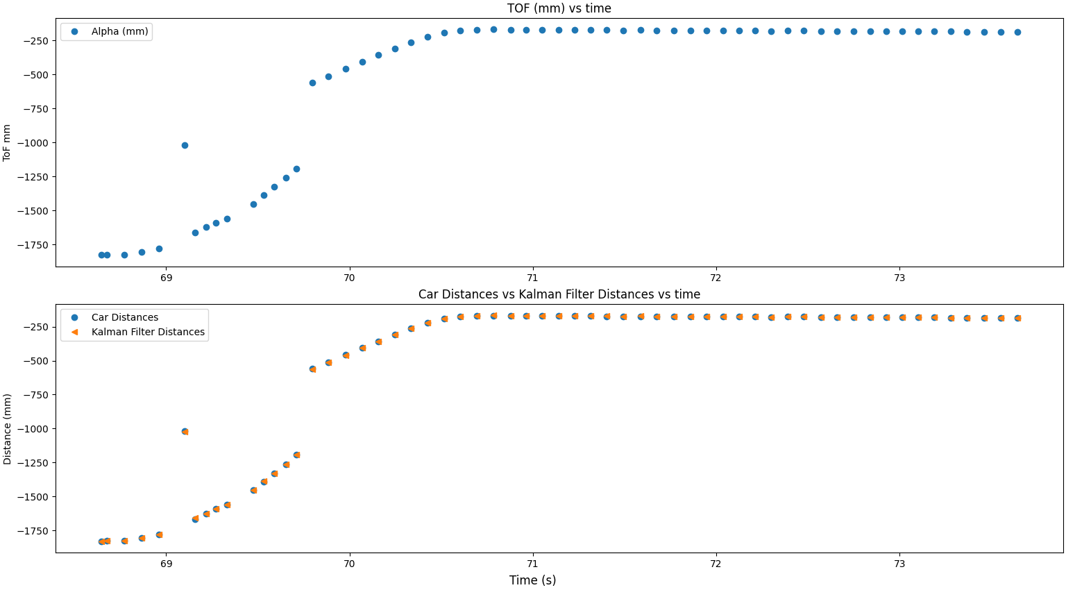
My third Kalman Filter output graph with the following variances:
- Process noise for distance: 100
- Process noise for speed: 100
- Sensor noise for the: 10
With these values, the sensor is trusted a lot more, and the Kalman Filter follows the sensor closely and follows the noise in the ToF data.
From the data above, I will reduce my trust in the sensor data by an amount between the first and second example. Here is my fourth Kalman Filter output graph with the following variances:
- Process noise for distance: 10
- Process noise for speed: 10
- Sensor noise for the: 40
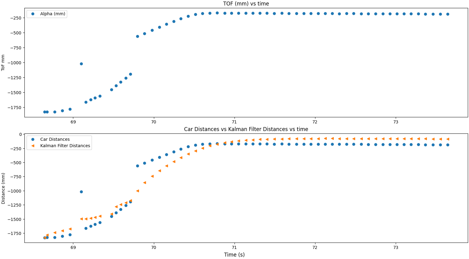
Now the Kalman filter is more robust to noise while still mostly following the sensor measurments.
Extrapolate ToF Task
I extrapolated the ToF data by getting the slope of the last two values then multiplying it by the time passed since the last value was recorded. I used the following code to get the extrapolated values from where I saved the ToF data and then fed it into the PID whenever data was unavailable.
I then ran the extrapolated ToF values through the Kalman filter and plotted the results. I used the code below to plot the results.
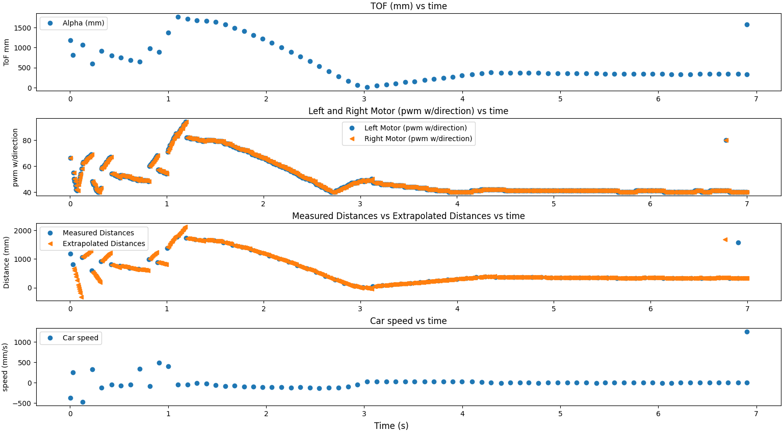
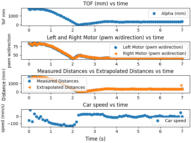
Here are three videos and graphs of the car moving and of the raw and estimated data in the same graph. As can be seen from the graphs, including the close up of the data, the ToF extrapolation managed to follow the ToF values very well and let the PID work as intended. Extrapolation did was influenced by noise, but this could be reduced by looking at the slope between more points.
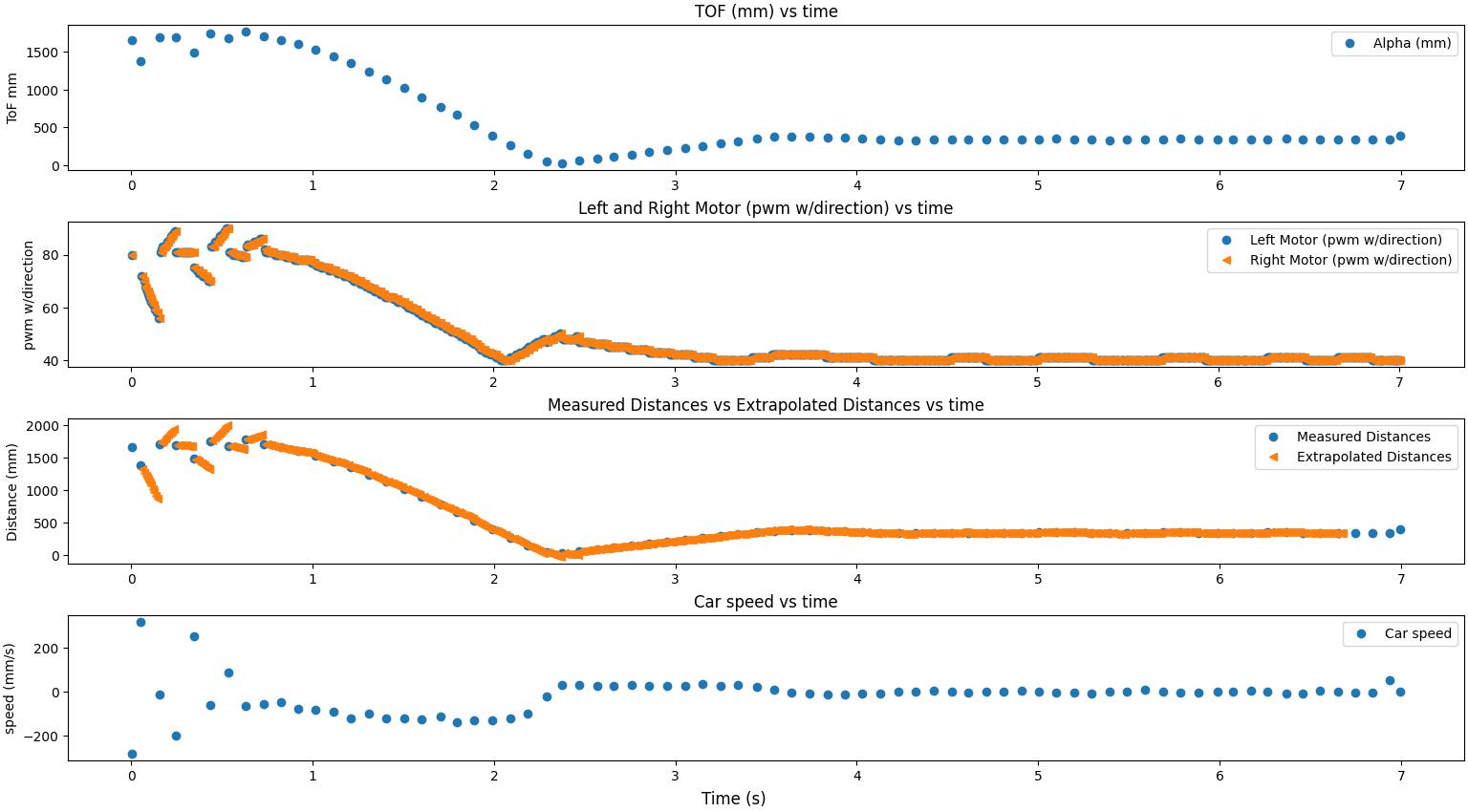
The close up of the extrapolated values and ToF values shows that the extrapolation is very close to the ToF values and follows them well.
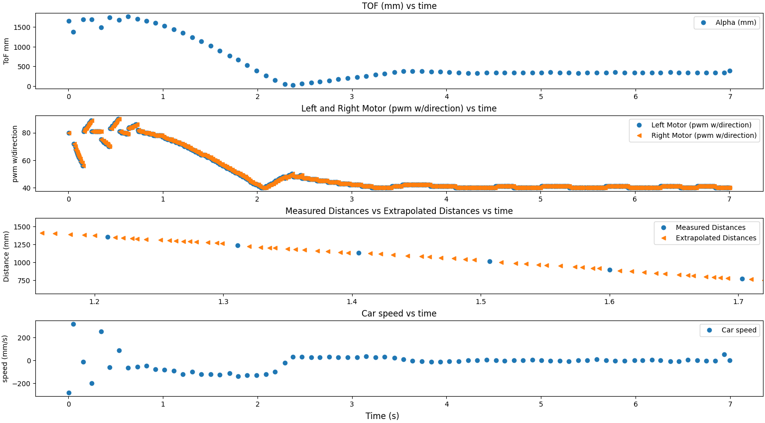
Here are the other two videos and graphs of the car using the ToF extrapolation.
